Introduction

In the first part of this series, we unpacked the big picture of scaling LLM training. The “why” and “what” behind ultra-scale setups, and how different forms of parallelism come together to make training trillion-parameter models even possible. That gave us the map.

Now it’s time to get into the weeds of the “how.” This second part is all about the practical side: choosing training configurations step-by-step, making trade-offs when you’re GPU-poor or GPU-rich, and squeezing every drop of performance out of the hardware. We’ll walk through memory fitting, batch sizing, throughput tuning, and then zoom in further to the GPU level — where kernel tricks, precision formats, and careful scheduling can make or break efficiency.

If part one was the strategy guide, part two is the playbook in action. Let’s dive in. It is highly recommended to read over the Hugging Face’s Ultra-Scale Playbook: Training LLMs on GPU Clusters to learn and use the details. I tried to curate a short version of the book to help you learn the concepts in a much shorter read before spending a few weeks to finish up the book.

Choosing the Best Training Configuration (Step-by-Step)

When setting up distributed training, consider a three-step approach:

Step 1: Fit the model in memory. First, ensure you can even hold a single training step in GPU memory. If you have a lot of GPUs (“GPU-rich”), you can distribute the model across them. For models up to ~10B, often one node (8 GPUs) with pure data parallel or tensor parallel is fine. For 10B-100B models, you may need to use 16+ GPUs. The options include tensor parallel (e.g. TP=8) combined with pipeline parallel, or TP=8 combined with ZeRO-3, or if communication allows, pure ZeRO-3 across enough GPUs(if you need a refresher on these concepts read part 1). At very large scale (hundreds of GPUs), pure DP/ZeRO-3 starts to bog down with comms, so introducing pipeline or tensor parallel groups is recommended. For example, at 512 GPUs, you might switch to something like TP=8 + DP (ZeRO-2) + maybe pipeline. The playbook suggests that at 1024 GPUs, a likely recipe is TP=8 + ZeRO-2 + Pipeline.

If you’re GPU-poor (limited GPUs for a large model), you fall back to the tricks we discussed: turn on full activation recompute (trading compute for memory) and increase gradient accumulation (trading time for memory). These allow training big models slowly with few GPUs.

Also, don’t forget special cases: if you need long sequences, consider adding context parallelism from the start (shard sequence across nodes). If using Mixture of Experts, plan to use expert parallelism to shard the experts across nodes.

The outcome of Step 1 is: you have a viable way to run a single forward/backward without OOM, using some combination of parallel strategies.

Step 2: Achieve the target global batch size. Once the model fits and runs, ensure you can reach the batch size you want for good model convergence. Perhaps after Step 1 your micro-batch is very small or your DP degree is limited. To adjust:

• If your current global batch is too small, increase it by either adding more data parallelism (more GPUs if available) or using more gradient accumulation steps. For extremely long sequences, you could also increase context parallelism (shard sequence more) to effectively allow larger batch per node.
• If your current global batch is too large (maybe you have more parallel workers than needed, causing overly large batch which might hurt convergence), you might reduce the number of data parallel replicas (and use other parallelism instead). Or reduce context parallel groups if sequence was over-sharded. Basically, dial down DP in favor of model-parallel approaches so that batch size per iteration isn’t excessive.

This step is about hitting the “sweet spot” batch size for model training. Often literature suggests using as large a batch as possible until loss starts to degrade. The playbook notes typical LLM pre-training batch sizes are in the tens of millions of tokens, and that has grown from 4M (LLaMA-1) to 60M (DeepSeek) as models and data grew. So you need to ensure your setup can reach those numbers. By tuning DP vs accumulation, you can get the exact global batch needed.

Now you have the model running at the desired batch size. The final step:

Step 3: Optimize training throughput. This is about speed – making sure the GPUs are utilized maximally and you are getting good hardware efficiency (high TFLOPs, minimal idle). Some guidelines from the playbook:

• Use tensor parallelism within nodes as much as reasonable, because TP can leverage fast intra-node links and speed up computation. Increase TP degree until you approach the number of GPUs per node (e.g. if 8 GPUs per node, TP=8 max). This reduces reliance on slower inter-node parallelisms.
• Increase data parallelism (with ZeRO) to use more GPUs for more throughput, but watch out for the point where communication overhead (grad all-reduce) starts hurting scaling. Up to some number of GPUs it’s fine, but beyond that consider switching strategy.
• When data parallel comm becomes a bottleneck (e.g. many nodes, network getting saturated with gradient sync), start using pipeline parallelism to split the model instead. Pipeline parallelism shifts to communicating activations (which might be less total bandwidth than syncing all grads for a huge model) and as noted can scale better across slow networks.
• Essentially, experiment with scaling each dimension one by one – try more TP, or more DP, or more PP, and see which yields better throughput. The optimal mix often needs empirical fine-tuning because it depends on hardware specifics (like your interconnect speed, GPU memory, etc.).
• Also, tune the micro-batch size. Larger micro-batches mean better GPU compute utilization (more arithmetic intensity per launch) but fewer pipeline micro-batches (if using PP) which means bigger bubble, and also larger memory usage for activations. Smaller micro-batches inversely. There is a sweet spot balancing compute vs communication overhead. Sometimes a slightly smaller micro-batch (with more grad accumulation) can allow overlapping communication more effectively, improving overall throughput.

The playbook basically encourages a systematic search which they in fact automated. They provided scripts in their Nanotron repository (check it out here) to sweep through many configurations and benchmark them. They themselves ran over 4,000 experiments (16k including test runs) exploring different parallelism combinations, model sizes from 1B to 80B, and cluster sizes from 1 to 64 nodes (8xH100 each). This huge search produced insights and the “optimal config” heatmaps for various scenarios.

One of the neat results is a heatmap of optimal configurations by model size vs number of nodes. In the following visualization, each cell lists the best combination of DP/TP/PP/etc and shows the achieved model FLOPs utilization (MFU) as color. A few observations stood out:

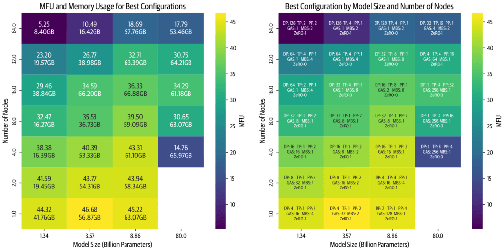
image source: ultrascale playbook

• Scaling inefficiency grows with more nodes: For smaller models especially, when you use many nodes (i.e. high total parallelism), efficiency drops. This is because small models don’t have enough computation to communication ratio, so adding more parallel workers just increases overhead without enough compute to hide it. They were also constrained by a fixed global batch of 1M tokens in the experiment, so they couldn’t just increase batch to utilize extra GPUs for tiny models.
• Large models on too few nodes run slow or don’t fit: For very big models, if you try to use only a couple of nodes, you either can’t fit the model at all or it runs at the edge of memory, causing lower speed. E.g. an 80B model on 4 nodes (32 GPUs) might technically fit with all tricks, but it will be painfully slow due to minimal memory headroom and a lot of recomputation or offloading.
• Implementation quality matters: They found that the relative performance of tensor vs pipeline parallel changed after optimizations. Initially their TP code was faster, but after optimizing pipeline code, pipeline became faster – then they improved TP comm overlap, and TP caught up again. The takeaway is that how well you implement these parallel strategies can affect which one is “better” on a given hardware. So always consider the maturity of the libraries you’re using.

They also share a candid look at the engineering challenges they faced when running thousands of distributed jobs. Real-world issues cropped up: PyTorch processes not freeing memory properly, Slurm terminating jobs causing node crashes, some runs hanging indefinitely. To get through the experiments, they had to do things like tune cluster restart times, parse NCCL debug logs to find bottlenecks, and optimize pipeline parallel performance specifically for multi-node. It underscores that distributed training at ultra-scale is not just theory – it requires a lot of practical debugging and engineering. Their team spent months sorting out these issues. So, even with the right configuration, ensuring stable and efficient training across a large cluster can be a challenge in practic. This is why open-sourcing these methods (through libraries like Nanotron or Megatron) is so valuable: it lets the community build on hardened implementations instead of reinventing the wheel and hitting the same pitfalls.

At this point, the playbook’s distributed training deep-dive concludes. They summarize that we’ve covered “5D parallelism” – all the major ways to slice the training problem across hardware. The final sections of the playbook then pivot to another crucial aspect: low-level GPU optimization. After all, once we distribute work, we also want to squeeze maximum performance out of each GPU by optimizing kernels, memory usage, and precision.

They make a great point: so far we assumed we can overlap communication and computation arbitrarily, but in reality, if both use the GPU’s same resources, they contend. Most GPU communications (like NCCL) use CUDA kernels under the hood, which occupy streaming multiprocessors just like compute kernels. So if you “overlap” all-reduce with backward compute, the all-reduce is actually stealing some GPU cycles and might slow down the backward compute a bit. Truly maximizing throughput thus requires understanding GPU internals: streams, concurrency, and perhaps techniques like using separate hardware engines for communication if available. This leads into topics like kernel fusion, multi-stream concurrency, and mixed precision.

So let’s briefly cover the highlights of optimizing on the GPU level from the playbook.

GPU-Level Optimizations: Fusing, Threading, and Mixing Precision

image source: https://blog.codingconfessions.com/p/gpu-computing

Modern GPUs (like NVIDIA’s) are incredibly powerful but to harness them fully you need to tailor your operations to the hardware. The playbook provides a quick primer on GPU architecture: An NVIDIA H100, for instance, has 132 Streaming Multiprocessors (SMs) with 128 CUDA cores each which is about ~16,896 cores total, and a hierarchy of memory from per-thread registers to shared memory (on-SM), L2 cache, and then high-bandwidth GPU memory (HBM). The gist: memory access speed varies widely (on-chip memory is far faster than HBM off-chip global memory), and GPUs like to run thousands of threads in parallel across those cores. To keep all those cores busy, you often need to launch operations in a way that exposes massive parallelism and minimizes waiting on memory.

FlashAttention: A Case Study in Kernel Optimization

One of the best examples of GPU-aware optimization in deep learning is FlashAttention. We discussed it briefly earlier in context of recomputation: FlashAttention was introduced by Tri Dao et al. and it reimplements the Transformer attention calculation to use GPU memory more efficiently. Normally, computing self-attention involves huge matrices (the Q·K^T scores matrix and the softmax probabilities) that are written to GPU’s global memory and read back for the value-weighted sum. That memory traffic is costly HBM, though high bandwidth (~>800 GB/s on H100), is still slower than on-chip memory by an order of magnitude. FlashAttention avoids ever materializing the big score matrix in HBM. Instead, it breaks the attention computation into tiles that fit in SM shared memory, computes partial softmax results on-the-fly, and only writes out the final outputs. It also cleverly only keeps track of minimal necessary statistics (like the max logits for softmax normalization) instead of the entire matrix. By doing this, FlashAttention reduces memory usage and reduces memory access overhead, turning attention into a more compute-bound (and cache-efficient) kernel.

The results were dramatic: FlashAttention became the default method for attention in many frameworks because it both lowers memory overhead and speeds up attention by 2-4x in practice. It essentially made those older attempts at approximate or sparse attention moot for many cases, since FlashAttention gives exact results with much better efficiency. The playbook notes that FlashAttention so thoroughly addressed the previous bottleneck that many research ideas (subquadratic attentions) fell by the wayside.

They also mention that the team didn’t stop at FlashAttention-1. FlashAttention-2 and -3 came out, further tuning performance: FA-2 reorganized threads and work to reduce non-matmul overheads and optimize memory transactions at an even finer level. FA-3 optimized for new hardware (Hopper GPUs) with FP8 and tensor core support. These improvements are less about changing the algorithm (still computing exact attention) and more about hand-crafting the kernel to better utilize GPU capabilities. For example, using tensor cores for more of the work, aligning memory access patterns with hardware, etc. It’s a testament that specialized kernels can provide huge gains. The downside is they might be specific (FlashAttention works for full attention with certain block sizes, etc.), which is why the playbook points to something called FlexAttention as a more flexible variant that can cover different attention masking patterns while still being fast.

FlashAttention demonstrates how understanding GPU memory hierarchy led to an innovation that removes a major bottleneck by trading compute for avoided memory I/O, a theme similar to activation recompute, but applied at the micro-kernel level.

Kernel Fusion and Scheduling

Beyond single-kernel innovations like FlashAttention, a more general GPU optimization is kernel fusion. Deep learning models often consist of many small operations strung together (e.g. linear -> bias add -> activation -> dropout). Launching a separate GPU kernel for each tiny op adds overhead (each launch has some fixed cost, and intermediate results go to memory). Kernel fusion combines multiple operations into one GPU kernel, so that data can stay in registers/shared memory between sub-operations and we launch fewer kernels overall. For example, fusing an elementwise add + GELU activation + dropout into one kernel means we load each element once, do add->GELU->dropout in one go, and write it out, instead of doing three passes. This saves memory bandwidth and launch overhead.

The playbook doesn’t explicitly walk through simple fusion, but it’s a known practice (libraries like Apex and JAX XLA do a lot of this under the hood). They do talk about overlapping compute and communication properly. One interesting note: overlapping isn’t always free because of contention on SMs. A possible advanced approach is to use dedicated communication engines (like NVIDIA’s NVLink/NVSwitch with NCCL’s SHARP or using network interface cards that can do RDMA). Future architectures may have more independent communication hardware to truly overlap without hitting SM usage.

Also, the playbook mentions a PyTorch team blog post on overlapping that might have introduced techniques like using multiple CUDA streams or tweaking priorities to better overlap comm/comp. The key is to ensure that while one kernel is using some SMs, another can use others (if possible), or to use asynchronous copy engines (like CUDA MemcpyAsync which can use copy engines). These are low-level details, but they matter for squeezing out every drop of performance.

Mixed Precision Training

Finally, a huge win in deep learning training efficiency has been mixed precision – using lower-precision numerical formats for most of the computation. By default, deep learning historically used 32-bit floats (FP32). But GPUs have special hardware (tensor cores) that can perform half-precision (16-bit) or even 8-bit matrix math at much higher throughput. Also, using 16-bit values halves memory bandwidth requirements and memory storage. Mixed precision training – using FP16 or BF16 for compute while maintaining enough stability can dramatically speed up training and reduce memory use, without sacrificing model quality when done right.

There are a few flavors of 16-bit: FP16 (float16) and bfloat16. FP16 has 5 exponent bits and 10 mantissa bits, bfloat16 has 8 exponent bits and 7 mantissa bits. The difference is bfloat16 has the same range as FP32 (due to more exponent bits) but less precision; FP16 has more precision but a narrower range (roughly 6 orders of magnitude vs 38 for bfloat16). Nvidia Volta/Turing/Ampere GPUs favored FP16, whereas Google TPUs and newer GPUs support BF16 natively, which is often easier to use (because BF16 doesn’t overflow on large values as easily, so you often don’t need loss scaling).

The playbook outlines three classic techniques introduced to make FP16 training as stable as FP32:

1. Maintain an FP32 master copy of weights. During training, you keep weights in FP32 as well, and update those with gradients (accumulating small changes accurately), while casting to FP16 for forward/backward computations. This avoids the issue of tiny weight updates being lost in FP16 precision (as FP16 might round small updates to zero).
2. Loss scaling. Gradients in deep networks can have very small values. To prevent FP16 underflow (gradients becoming zero), you multiply the loss by a large constant (e.g. 1024) before backprop, so all gradients are scaled up into a representable range, do backward in FP16, then divide the gradients by the scale to restore them. This technique is automated in frameworks (AMP: Automatic Mixed Precision).
3. FP32 accumulation for certain operations. Some reductions (like summing a large array of FP16 numbers) can overflow or lose precision. The solution is to do those in FP32 internally. For example, when accumulating gradients across batches or computing running averages, use higher precision for the accumulation.

With these, FP16 training can achieve the same accuracy as FP32 in most cases, while using half the memory for activations/gradients and often running faster (up to 2x speed if compute-bound by matmuls, thanks to tensor cores).

Even more exciting, the latest NVIDIA H100 GPUs introduced support for FP8 precision. Two FP8 formats (e4m3 and e5m2) are defined with 8 total bits. FP8 halves the precision of FP16 and again offers potentially double the speed for matrix ops. In fact, H100’s theoretical FLOPs in FP8 are twice that of BF16. The lure is huge: if we can train in 8-bit, we might double throughput again and cut memory by 50% again.

However, FP8 training is on the cutting edge. The playbook notes it’s experimental as of early 2025. The big issue is stability – with such low precision, models often diverge (loss blows up or NaNs) if you naively train. Research efforts (NVIDIA’s Transformer Engine, the FP8 for Large Models (FP8-LLM) paper, and Hugging Face’s own experiments in DeepSeek-V3) have shown it is possible to train large models in FP8, but you need many tricks:

• Keep some computations in higher precision. E.g. in NVIDIA’s transformer engine, they do matrix multiplies in FP8 but keep the accumulation in FP16, and some parts like layer norm in FP16/32. DeepSeek-V3 reported using FP8 for most, but keeping a lot of stuff in BF16/FP32 as needed.
• Normalize activations dynamically. One big approach is having an exponent “scale” per group of values to account for outliers. DeepSeek-V3 did per-128x128 tile scaling: they compute the max absolute value in that tile of activations or weights, and use it to choose a scale so that values utilize the FP8 range optimally. This is essentially a form of adaptive quantization that prevents one outlier from forcing everything else to zero in FP8.
• Loss scaling might still be needed, and other stability tricks like clipping gradients, or adjusting optimizer hyperparameters.

The playbook provides a table comparing some known FP8 training approaches. For example, one approach (IBM’s FP8 paper) got ~55% memory reduction vs BF16 by doing FP8 for matmuls but still using FP16 for some accumulations. DeepSeek-V3 achieved ~25% reduction vs BF16 (they were conservative to maintain stability). Another approach from NVIDIA (“Nanotron’s FP8” in the table) claims 50% reduction with their own mix of BF16/FP8 usage. The point is, FP8 can save another big chunk of memory and compute, but it’s still evolving. The authors expect FP8 will become the standard in the near future, potentially replacing BF16, once these methods mature. And looking further, NVIDIA has already announced that their next-gen GPU (Blackwell) will even support FP4 training which sounds crazy now, but so did FP16 a few years ago!

The journey the playbook takes us on is pretty incredible. From single-GPU basics through all dimensions of parallelism, and down into the guts of GPU kernels and number formats, it provides a comprehensive view of how to train large language models efficiently.

Conclusion

Bringing it all together: training massive LLMs efficiently is about combining many strategies, from algorithmic tricks like recomputation and mixed precision to distributed parallelism across every possible dimension to wring the most out of expensive GPU clusters. In this post we followed the Hugging Face Ultra-Scale Playbook through these techniques. Starting with a single GPU handling a simple model, we escalated to coordinating thousands of GPUs to train models like Llama-3 70B or DeepSeek-V3. Along the way, we learned how to overcome memory limitations (shard and recompute whatever you can), how to keep GPUs busy with data/model parallel work (overlap communication, use all levels of parallelism), and how to optimize the computations themselves (fuse kernels, use FlashAttention, and leverage lower precision). By the end, terms like “5D parallelism” or a diagram of Llama-3’s 4D parallel setup don’t seem so intimidating and we can understand how each dimension plays a role.

One striking message is that these techniques are not just for billion-dollar labs anymore. As the open-source community and model sizes both grow, distributed training know-how is increasingly important for everyone. Fine-tuning or serving large models also benefit from these same techniques, so a wider swath of engineers and researchers will need to be comfortable with them. It’s becoming part of the standard toolkit for AI developers.

The Ultra-Scale Playbook is essentially an open-sourced compilation of hard-earned knowledge from running those thousands of experiments and months of debugging on real clusters. Hugging Face sharing this “secret sauce” is a big win for open science and the community. It lowers the barrier for others to build on top of state-of-the-art methods.

There’s always more to learn (the playbook includes references to many papers and suggests implementing things yourself or contributing to frameworks to really master this). But I hope this narrative overview has given a cohesive understanding of large-scale LLM training techniques. In the future, we’ll likely see even more automation (tools that auto-parallelize models), better libraries, and perhaps new paradigms (like training on specialized hardware or using robust sharding algorithms so we hardly think about it). For now, though, if you’re looking to train the next 100B+ model, the strategies discussed here and in the playbook are your bread and butter.