Introduction

Training today’s largest language models demands massive computational resources, often thousands of GPUs humming in perfect harmony, orchestrated to act as one. Until recently, only a few elite research labs could marshal such “symphonies” of compute power. The open-source movement has started to change that by releasing model weights (like Llama or DeepSeek) and technical reports, but the know-how of coordinating hundreds of GPUs to train these massive models remains complex and fragmented across papers and private code bases.

Hugging Face’s Ultra-Scale Playbook: Training LLMs on GPU Clusters is an open-source guidebook aiming to demystify this complexity. This was my motivation to write a short summary of it. Most of the curated content here comes from the free book Huggingface kindly put together with a few tweaks. The book starts from the basics and walks through how to scale training from a single GPU to tens, hundreds, and even thousands of GPUs, illustrating concepts with code examples and real benchmarks. In this post, I’ll summarize key insights from the playbook covering why large-scale training is challenging and how a suite of techniques (data, tensor, pipeline, and context parallelism, plus ZeRO, mixed precision, etc.) can be used to meet these challenges. The goal is to provide a coherent narrative of how we can train high-performing LLMs efficiently with distributed computing.

Before diving in, the playbook emphasizes three recurring challenges in scaling training:

• Memory usage: If the model or batch doesn’t fit in GPU memory, training can’t proceed. Managing memory is a hard limit we must overcome for large models.
• Compute efficiency: We want GPUs doing math, not sitting idle or waiting on data. So we must keep GPUs busy and reduce any stalls.
• Communication overhead: In multi-GPU setups, GPUs need to exchange data (gradients, parameters, activations). Communication time can eat into our training throughput, so minimizing or overlapping it with computation is crucial.

All the techniques we’ll discuss target one or more of these issues. Let’s start at the beginning: how do we even train a large model on one GPU without running out of memory or wasting compute? This will set the stage for scaling out to many GPUs.

---

Training on One GPU (Memory and Batch Size)

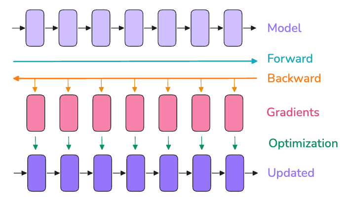
image source: ultrascale playbook

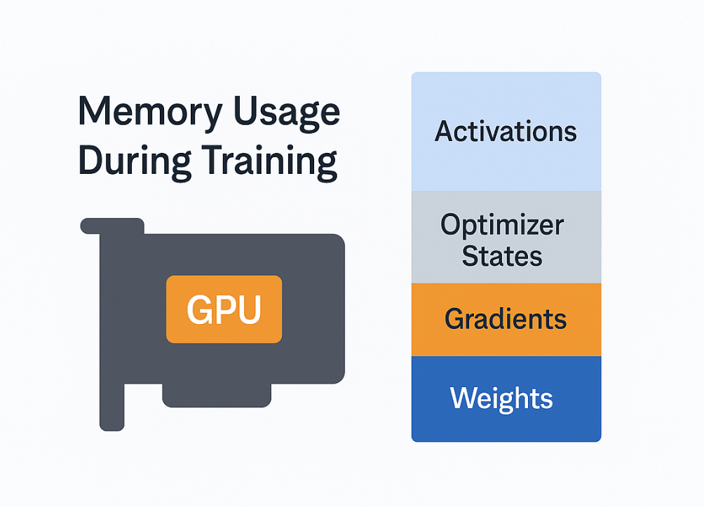
Even a single GPU can face memory bottlenecks when training large models or using large batch sizes. To understand why, consider what occupies GPU memory during training:

• Model weights: the parameters of the neural network.
• Gradients: the gradients for each weight computed during back propagation.
• Optimizer states: e.g. for Adam, momentum and variance for each weight.
• Activations: intermediate outputs from forward passes needed to compute gradients in the backward pass.

These components all consume memory. As models and batches grow, memory usage can explode, leading to out-of-memory (OOM) errors. For instance, if you try to fit millions of tokens in a batch on one GPU, you’ll likely hit a wall.

Profiling memory usage during a training step reveals a typical pattern: during the forward pass, activations allocate a lot of space; during the backward pass, gradients accumulate and activations get freed as we go; finally, the optimizer step adds more memory usage for momentums/variances. The first training iteration often uses extra memory due to PyTorch’s CUDA memory allocator warming up, which is why sometimes step 1 succeeds but step 2 OOMs as optimizer state appears. The key takeaway is that activation memory scales with batch size and sequence length, often becoming the largest chunk for long sequences. Meanwhile, weights, grads, and optimizer state scale with model size but not with sequence length or batch tokens.

To tame memory usage on one GPU, the playbook introduces two fundamental techniques: activation recomputation and gradient accumulation.

Activation Recomputation (Gradient Checkpointing)

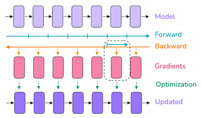
image source: ultrascale playbook

One culprit of memory bloat is storing every activation for backprop. Activation recomputation (also known as gradient checkpointing or rematerialization) trades computation for memory: instead of keeping all intermediate activations, we drop some activations during the forward pass and recompute them on-the-fly during the backward pass. By only caching a few “checkpoint” activations (say, one per layer or per block of layers), we dramatically cut the activation memory footprint at the cost of doing some extra forward calculations in backward. Essentially, we redo parts of the forward pass in order to avoid storing large activation tensors in memory a very worthwhile trade-off when memory is at a premium.

There are different strategies for choosing what to recompute. The full strategy checkpoints between every single layer (maximal memory saving, but adds ~30-40% more compute time). A smarter selective strategy (from the original NVIDIA paper on recomputation) found that the largest activations with cheapest recompute are in attention layers, so one can choose to recompute those while still storing other expensive parts like feed-forward activations. For a 175B model (GPT-3), selective recompute saved ~70% of activation memory at only ~2.7% extra compute cost which is a huge win. In practice, modern implementations like FlashAttention actually integrate recomputation: they recompute attention softmax results on the fly in backward instead of storing them, implicitly using selective activation recompute. The bottom line: activation checkpointing is now standard for training very large models, because it significantly cuts memory usage with only a minor hit to training throughput. Often, the memory savings even enable faster training overall, since GPUs can avoid running out of fast memory and spend less time shuffling data to slower memory.

Gradient Accumulation

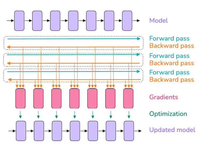
image source: ultrascale playbook

Even with recomputation, a single GPU might not hold a very large batch of data. Gradient accumulation is a straightforward workaround: split your batch into several micro-batches that do fit in memory, run forward and backward on each micro-batch sequentially, and accumulate the gradients before applying one optimizer step at the end. In effect, if you want a “global batch size” of N but can only fit n per pass, you can do N/n passes (micro-batches of size n) and sum up gradients so that one update sees N total examples. This yields the same math as a big batch of size N, while avoiding memory explosion during any single forward pass. The trade-off is of course time. The gradient accumulation processes batches serially on one device, so training takes longer than if we could process them in parallel. However, it allows you to reach a desired effective batch size even with limited memory.

In practice, you choose a micro-batch size (mbs) that fits in GPU memory and a number of accumulation steps such that global_batch = mbs * grad_accum_steps. For example, if you want a batch of 1024 samples but can only fit 256 at once, you can accumulate 4 micro-batches (256 each) to get the effect of 1024. Generally, it’s best to use as much parallelism as possible (bigger data parallel size, which we’ll discuss next) and use gradient accumulation to make up the rest, since accumulation is purely sequential. But when GPUs are the limiting factor, gradient accumulation is your friend to reach large batch sizes without OOMs.

Using activation recompute and gradient accumulation, one GPU can now handle larger models and batches than naive training would allow. We’ve essentially traded extra computation and time to alleviate memory limits. At this point in the playbook’s story, we can successfully train a model (albeit slowly) on a single GPU. The next logical step is scaling out to multiple GPUs to accelerate training. This introduces new challenges: how to split the work across GPUs and how to manage the communication and synchronization between them efficiently. The simplest approach is data parallelism, so let’s start there.

Training on Multiple GPUs

Data Parallelism: Scale Out by Splitting the Data

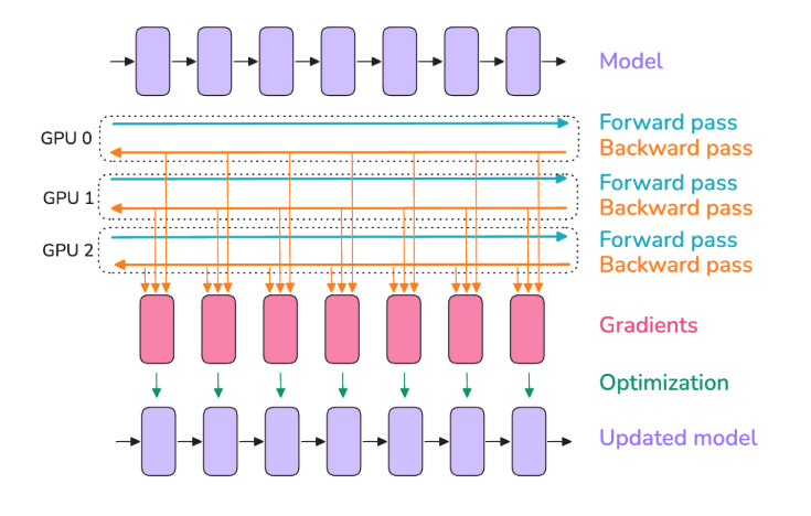
image source: ultrascale playbook

Data parallelism (DP) is the classic way to use multiple GPUs for training. The idea is simple: copy the entire model to each GPU, feed each GPU a different subset of the data (micro-batches), and combine their results. In practice, each GPU computes forward and backward on its own micro-batch, producing gradients specific to its data. Then we perform an all-reduce operation to average gradients across all GPUs, so that all model replicas stay in sync. After this synchronization, each GPU has the same averaged gradients and can proceed to update its copy of the weights identically. The result is as if you had processed a bigger batch equal to the sum of all the micro-batches (one per GPU) in parallel, hence boosting throughput almost linearly with the number of GPUs, in theory.

Key point: Data parallelism increases throughput by using more GPUs to process different data in parallel, but it does not increase per-GPU memory requirements for the model; each GPU still has a full model copy and handles a full micro-batch. So DP by itself doesn’t help fit a larger model on a GPU; it helps train faster by leveraging more GPUs on more data. (We will handle model partitioning with other techniques soon.) The only memory relief DP provides is that, for a given global batch, each GPU gets a fraction of it. For example, if 4 GPUs are data-parallel, a batch of 1024 is split into 4×256 micro-batches, so activations per GPU are as if batch=256, which is easier on memory. In other words, data parallelism acts like increasing gradient accumulation but doing the micro-batches concurrently on multiple GPUs instead of sequentially. This is why typically one tries to maximize DP (parallel work) before relying on too much gradient accumulation (sequential work).

However, naively implementing DP can introduce a new bottleneck: the gradient synchronization step. If we wait until after each GPU finishes its entire backward pass to then do an all-reduce of all gradients, we end up with a big sequential gap; all GPUs sit idle during the communication phase. This is bad for efficiency, as it stalls our expensive hardware. The playbook calls such sequential “compute then communicate” a big no-no. Instead, we apply a series of optimizations to overlap communication with computation and reduce overhead:

• Overlap gradient synchronization with backward computation: Don’t wait for the whole backward pass to finish before syncing grads. As soon as each layer’s gradients are computed, we can start an all-reduce for that layer in the background, while backward continues computing gradients for earlier layers. In PyTorch, this is done by attaching asynchronous communication hooks to parameters as soon as a grad is ready, it begins summing with other GPUs. This way, much of the gradient all-reduce communication happens concurrently with the backward pass that’s still running, meaning by the time backprop is done, a lot of the gradients are already averaged across GPUs. This significantly cuts down idle time. Essentially, computation and communication are pipelined instead of serial.
• Bucket gradients to communicate in larger chunks: Instead of launching one all-reduce for each small gradient tensor, we combine many gradients into bigger buckets and all-reduce those. Fewer large messages are more efficient than tons of tiny ones. Think of it like sending a few big packages rather than many little envelopes, there’s overhead to each send/receive, so bigger transfers amortize that overhead. Frameworks like PyTorch’s DDP (DistributedDataParallel) do this by default: they’ll group gradients and perform grouped all-reduces.
• Combine with gradient accumulation smartly: If we are using gradient accumulation and data parallelism together, we should avoid unnecessarily syncing gradients after every micro-batch. In a naive approach, if you have DP on 4 GPUs and do 4 accumulation steps, one might accidentally all-reduce after each of the 4 micro-batches, which isn’t needed we only need to all-reduce once at the end of the full batch accumulation. The solution is to suppress gradient syncing during intermediate accumulation steps and only sync after the final one. In PyTorch, one can wrap model.no_sync() around the first (N-1) backwards and let only the last backward trigger the all-reduce. This avoids redundant communications during accumulation.

With these optimizations, data parallelism becomes much more efficient. We essentially achieve near-perfect linear scaling for a while, e.g. 8 GPUs can handle ~8× the data per step of 1 GPU, with only a small overhead from overlapping comms. However, as you keep increasing the number of GPUs, communication can still become a bottleneck eventually. The playbook notes that at very large scale (e.g. 512+ GPUs), even with overlaps, the gradient all-reduce may start to lag due to network latency and bandwidth limits. At some point, adding more GPUs yields diminishing returns because the coordination cost dominates. In their experiments, beyond a certain point, throughput actually decreases if we keep scaling pure data parallelism. This tells us data parallelism alone isn’t sufficient for massive scale we’ll need to introduce other parallelism dimensions to handle very large models or very large GPU counts.

Before moving on, let’s recap the state of our training setup so far: We can train a model on one GPU with recomputation and accumulation. We can train faster on multiple GPUs with data parallelism, cleverly overlapping communications. But data parallelism still assumes each GPU holds a full copy of the model. What if the model is so big that it can’t even fit on one GPU’s memory? For example, today’s 70B+ parameter models (or future 1T models) might exceed the 80 GB memory of even a high-end GPU once you include optimizer states and activations. We have indeed run into such cases – the playbook says “larger models often don’t fit into a single GPU, even with activation recomputation”. If your model’s parameters alone are, say, 140 GB (which a 70B model in FP16 roughly is, since 70B * 2 bytes ≈ 140B bytes ~ 130 GiB), you clearly need more than one GPU’s memory to hold it.

This is where model parallelism techniques come into play. Model parallelism means breaking up the model itself across multiple devices, instead of replicating it. The playbook covers multiple forms: tensor parallelism, pipeline parallelism, sequence (context) parallelism, and expert parallelism. These can be combined with data parallelism (and with each other) in various ways. Hence the term “5D Parallelism” for the five dimensions (DP, TP, PP, CP, EP) that advanced setups may utilize. We’ll explore each briefly.

Model Parallelism Part 1: Tensor Parallelism (Splitting Layers)

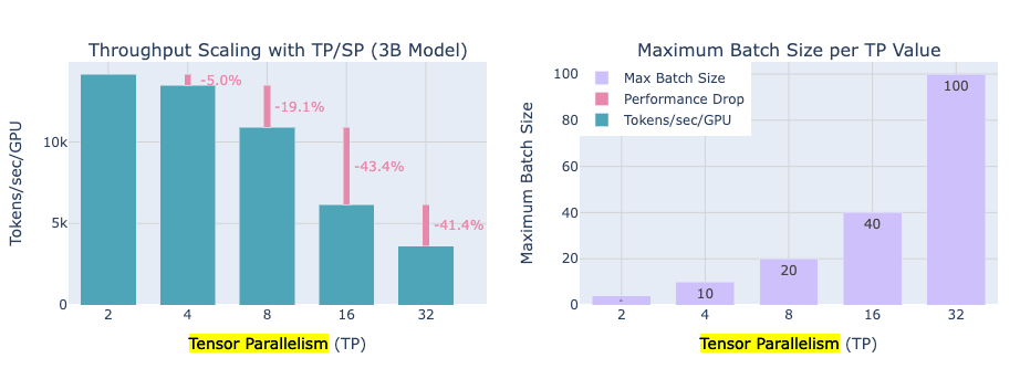
image source: ultrascale playbook

Tensor Parallelism (TP) refers to splitting the computations within each layer of the neural network across multiple GPUs. Instead of each GPU having a full copy of the model, each GPU holds a partition of the model’s weights and computes a partition of the output. By coordinating, they produce the same result as the full model. In essence, TP leverages the linear algebra structure of neural networks: large matrix-matrix multiplications can be split into smaller pieces. For example, if a layer does X @ W (matrix multiply of input activations X by weight matrix W), we can split either the weight matrix’s columns or rows among GPUs, do partial products, and then exchange results:

• If we split W by columns (column-parallel), each GPU gets a subset of output features. We broadcast the full input X to all GPUs (so each can multiply its piece of W), then all-gather the partial outputs from GPUs to form the complete output (Broadcasting inputs and gathering outputs).
• If we split W by rows (row-parallel), each GPU holds a chunk of input features. We scatter (partition) the input X among GPUs, each multiplies its chunk of X with its chunk of W, and then we all-reduce (sum) the results because each GPU’s output now is a partial sum needed for the full output(Scatter inputs, sum outputs).

These are two fundamental modes (often both are used in different parts of a layer). In practice, frameworks like Megatron-LM implement a mix: e.g. for a Transformer’s feed-forward network, you might do the first linear layer in a column-parallel way (split output units) and the second linear in row-parallel way (split input units). This combination ensures that intermediate synchronization can be minimized (they avoid an extra all-reduce between two splits by choosing the right order). In multi-head attention, splitting by columns corresponds to giving different GPUs different attention heads to compute (since heads are independent), which is a very natural form of tensor parallelism for attention. The output projection can be row-splitted. In short, tensor parallelism slices up the heavy linear algebra operations and distributes them, so each GPU handles a fraction of the neurons or attention heads.

Benefits: Each GPU now stores only its fraction of the weights (and activations), so memory per GPU is reduced. If you have 4 GPUs in a tensor-parallel group, each might hold ~1/4 of the model parameters and process 1/4 of the activations for those layers. This can make an enormous model fit into one node, e.g. the playbook notes that going from TP=1 (no splitting) to TP=8 (8-way split) let them fit a 70B model on 8×80GB GPUs in one node where it otherwise wouldn’t.

Trade-offs: Tensor parallelism introduces communication in the middle of layer computations, and these communications (the all-gathers and all-reduces) cannot be entirely hidden by computation. Unlike data parallel grad sync, which happens after compute (and we managed to overlap much of it), TP’s communication is in the critical path of the forward/backward pass. For instance, an all-reduce is needed to sum partial results before a layer’s computation can proceed to the next step, creating an unavoidable synchronization point. This means as you increase the number of GPUs in a TP group, the communication overhead grows – and at some point, adding more GPUs (especially across slower interconnects) will hurt scaling efficiency. The playbook observed sharp diminishing returns beyond 8 GPUs for tensor parallelism; going to 16 or 32 GPUs (spanning multiple nodes without NVLink) led to significant drop in speed because network communication dominated the gains from splitting work. Conclusion: TP is most effective within a node (where GPUs have fast links) and for moderate splits, but it doesn’t infinitely scale across many nodes due to comm overhead.

Despite that, TP is a vital tool. It solves the problem of very large model size by partitioning weights, which DP couldn’t. Often, TP is used in conjunction with DP: e.g. if you have 8 GPUs per node, you might do TP across the 8 GPUs of a node (so each node holds one full model in aggregate), and then use DP across multiple nodes (each node running a copy of the model in TP form). This confines the high-bandwidth requirement of TP to inside nodes and uses DP (which tolerates slower networks better, thanks to overlapping) across nodes.

One more extension: Sequence Parallelism (SP). This is a companion to tensor parallelism introduced to handle certain layers like layer norm and dropout. In a Transformer, layer normalization and dropout at the end of a layer require the full hidden state to compute (layer norm needs the mean/variance of the entire vector). In pure TP, after splitting the hidden dimension, each GPU had only part of the vector, so one naive approach would gather the whole vector on each GPU to do layer norm which would temporarily negate the memory savings. Sequence parallelism instead says: for those troublesome ops, split the sequence dimension among GPUs instead of hidden. That way, each GPU has a full (un-sharded) hidden vector for a subset of the sequence positions, and can compute layer norm or dropout locally on its chunk. After that, GPUs exchange data as needed to go back into tensor-parallel splits for the next linear layer. Essentially, SP shards the activations for certain layers along the sequence length. This keeps memory distributed and avoids ever assembling a full large activation on one GPU. The net effect is that the maximum activation size each GPU sees is reduced – either we split by hidden (TP) or by sequence (SP) for any given part, so we never hold a full batch_size x seq_length x hidden activation on one device. It’s a bit complicated to implement (lots of careful all-gathers and reduce-scatters when transitioning between TP and SP regions), but it further pushes down memory usage and works hand-in-hand with TP. Note: The playbook uses “sequence parallelism” in this specific sense tied to TP. To avoid confusion, they call the other concept of splitting extremely long sequence across GPUs context parallelism.

At this stage, we have tools to split a model within one node (TP+SP) and to replicate across nodes (DP). But what if our sequence length is enormous, like 128k tokens? Even with activation recompute, attention with such a long sequence might blow up memory. This is where Context Parallelism enters.

Model Parallelism Part 2: Context (Sequence) Parallelism for Long Sequences

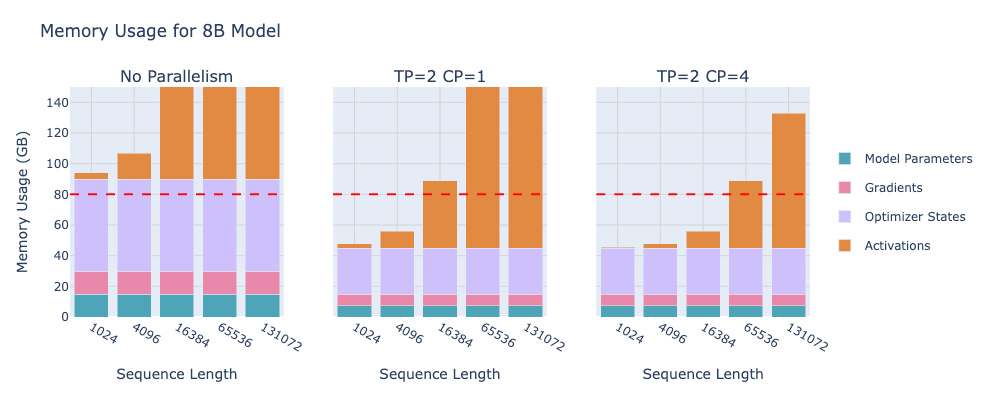
image source: ultrascale playbook

Context Parallelism (CP) is effectively splitting long sequences across multiple GPUs, to deal with cases where one GPU’s memory can’t handle the attention context. If you have, say, 128k token sequences, even after doing TP on your layers, the attention mechanism still needs to attend over 128k tokens, which on a single node could be infeasible memory-wise. CP extends the idea of sequence parallelism from the previous section but at a larger scale: it shards the entire model’s sequence processing across GPUs. Each GPU gets a chunk of the sequence (e.g. GPU1 handles tokens 1-32k, GPU2 handles tokens 32k-64k, etc.), and they work together to compute attention over the full sequence length.

For most parts of the model, splitting by sequence is actually trivial, e.g. in feed-forward layers or embedding layers, each token’s computation is independent of others, so each GPU can handle its subset without talking to others. Gradients are synced after (much like DP) by an all-reduce across those context-parallel GPUs. The tricky part is the self-attention layer, because attention is global: every token’s attention weight can attend to every other token’s key/value. If we’ve divided tokens among GPUs, then each GPU initially only has the keys/values for the tokens it owns, but to compute attention properly, it needs keys/values from all tokens. A naive approach would gather all keys/values on every GPU (like an all-gather of sequence parts), but that would be a huge communication (and memory) cost. Instead, the playbook highlights a more efficient approach called Ring Attention.

Ring Attention is an all to all communication pattern tailored for attention. Imagine GPUs arranged in a ring; each GPU sends its chunk of keys/values to the next GPU, while computing partial attention scores on the chunk it currently has. They do this in stages, passing chunks around the ring. The idea is that at any time, a GPU is busy computing attention on some portion of the sequence while simultaneously receiving the next portion from a neighbour (overlapping comm with compute). By the time it finishes computing with one chunk, it has received the next chunk to process, and so on, until it has cycled through all chunks of the sequence. This way, no GPU ever had to hold all 128k tokens’ keys/values at once – it only stores one chunk at a time (greatly saving memory). And the communication is spread out over multiple smaller transfers (each step of the ring) which are overlapped with compute.

However, a naive ring order for causal attention (where each token only attends to earlier tokens) can lead to load imbalances. The playbook describes how in a straightforward scheme, the first GPU might finish its work early while others are still crunching, due to how the attention mask looks. To fix this, they mention Zig-Zag (Striped) Ring Attention, which basically shuffles which token blocks go to which GPU so that each GPU gets a mix of early and late tokens, balancing the workload. Without going into deep detail: ZigZag ensures each GPU has a similar amount of actual attention computation, preventing one from finishing far before the others. The result is a nicely balanced, efficient ring-based attention that scales to extremely long contexts across multiple GPUs.

With context parallelism, the playbook demonstrated they could handle sequence lengths that would otherwise be impossible on a single node (like >100k tokens) by distributing the sequence. CP complements tensor parallelism: we might use 8 GPUs per node in TP to handle model size, and then use multiple nodes in CP to handle sequence length beyond what one node can do. And importantly, CP’s overhead is mostly in the attention comms, which (thanks to ring attention) are efficiently overlapped with compute. After using CP, extremely long sequences become tractable at the cost of some extra communication, but that’s preferable to not training on long sequences at all.

Model Parallelism Part 3: Pipeline Parallelism (Layer-wise)

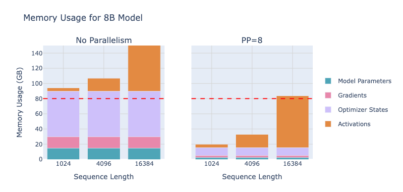
image source: ultrascale playbook

So far we’ve scaled within layers (TP) and across sequences (CP). Another orthogonal axis is Pipeline Parallelism (PP) – splitting the model by layers across different GPUs. For example, if you have 4 GPUs, you could put the first quarter of the model’s layers on GPU1, the next quarter on GPU2, and so on. Then when you do a forward pass, GPU1 processes the input through layers 1-N, sends the intermediate activations to GPU2 which does layers N+1-2N, and so forth, like a multi-stage. The same happens in reverse for back propagation. In effect, each GPU stores only a portion of the model’s layers, which is great for memory: a model too big for one GPU might easily be stored in pieces on 4 GPUs. In fact, pipeline parallelism, like ZeRO-3 , is one of the main ways to train giant models that no single GPU (or single node) can hold.

However, pipeline parallelism introduces a new challenge: pipeline bubble (idle time). If we naively do it, the first GPU does forward pass on layer1-… then layerN and passes to GPU2, etc., and in backprop the last GPU goes last – this means at any given time, not all GPUs are being used. For example, at the very start, GPU1 is busy with the first micro-batch’s forward, while GPUs 2-4 are idle waiting for data. At the very end, GPU4 is finishing the backward on the last micro-batch while GPUs 1-3 are idle. This sequential nature leads to idle periods represented as the “pipeline bubble.” If we only process one batch at a time through the pipeline, the utilization diagram looks terrible – lots of idle time. The efficiency of pipeline parallelism is typically measured by how much of this bubble time we can eliminate.

The good news: we can fill the pipeline with multiple micro-batches in flight. Instead of doing one batch forward then backward fully, we can send in a new micro-batch every time the first stage is free. The simplest version of this is the “all forward, all backward” (AFAB) schedule: first, feed m micro-batches one after the other into the pipeline (so the first stage sees m forwards one after another, the later stages always have something to do after the pipeline is filled), then after the last forward is done, initiate the backward passes for each micro-batch in sequence. In AFAB, if you have p pipeline stages and m micro-batches, the bubble (idle time) ratio is reduced to (p-1)/m instead of p-1. By increasing the number of micro-batches m, the bubble shrinks proportionally. Essentially, more micro-batches = more overlap between stages = better efficiency. In the limit of very many micro-batches, pipeline approaches full utilization (except a small fraction).

However, AFAB has a downside: memory usage. In that schedule, we did all forwards first then all backwards. That means during the forward phase, none of the backwards have started, so we are storing all those micro-batches’ activations for the backward pass later. If m is large, the activation memory can explode (we kept activations for m micro-batches). This could negate the memory advantage of pipeline parallelism. To mitigate this, researchers came up with the 1F1B (One Forward One Backward) schedule. In 1F1B, after an initial fill, the pipeline runs by alternating one forward, one backward at each step. In steady state, every time a new micro-batch forward enters the first stage, a finished micro-batch’s backward is computed on that stage, etc., interleaving forward and backward passes. This means we don’t need to store all m activations; at most we keep activations for roughly p micro-batches (the pipeline length) before they start getting released by backward. So 1F1B significantly reduces activation memory vs. AFAB, it’s much more memory-friendly for deep pipelines. The trade-off is that 1F1B doesn’t actually reduce the bubble size inherently (the bubble still exists, but now we can afford to use more micro-batches m to shrink it, since memory is less of a constraint).

Implementing pipeline schedules like 1F1B is non-trivial – it requires careful coordination so each GPU knows when to switch from forward to backward on a given micro-batch, etc., which complicates the training loop code. But libraries (like DeepSpeed or Megatron) handle this under the hood. The playbook’s benchmarks show that with a decent number of micro-batches (say m = 32) the pipeline bubble can be made relatively small except at extremely large pipeline parallel degrees. Interestingly, they found pipeline parallelism scales across nodes better than tensor parallelism: e.g. going from 1 node to 2 nodes (8 to 16 pipeline stages) only dropped throughput ~14%, whereas doing the same with tensor parallelism might drop ~43%. That’s because pipeline sends only moderate-size activation tensors between stages, a few times per micro-batch, which is easier on inter-node bandwidth than TP’s frequent all-reduces. This makes pipeline parallelism attractive for multi-node scaling, as it tolerates slower interconnect better.

To push efficiency further, the playbook discusses even fancier pipeline schemes: Interleaved Pipelines and “Zero Bubble” techniques. The idea of interleaving is to cut each GPU’s share of layers into multiple chunks (say GPU1 has layers 1,3,5,7 and GPU2 has 2,4,6,8, etc.) and loop micro-batches through them in a round-robin fashion. This increases the “virtual” pipeline length (a micro-batch might go through the same GPU multiple times for different layers in an interleaved fashion) and can reduce bubble by effectively having v pipeline stages per GPU. There’s a cost of extra communication because a micro-batch might travel between GPUs more times, but it can significantly reduce idle time when done well. Additionally, research ideas like DualPipe aim for zero bubble, meaning two pipelines operate in parallel offset by half a cycle to eliminate idle time. These are advanced optimizations and typically require complex coordination. They are beyond the scope of an overview, but the trend is: clever scheduling can nearly eliminate pipeline idle time at the cost of complexity and sometimes more communication.

With pipeline parallelism, we have another powerful tool to distribute a model that’s too large for one node (or even one rack). It’s often compared to ZeRO-3 (which shards model weights as well) because both tackle the challenge of model size by partitioning parameters. The playbook provides a nice comparison: pipeline parallelism splits layers so each GPU holds a contiguous chunk of the model, whereas ZeRO-3 (described next) shards every layer’s weights across GPUs. Pipeline sends activations between GPUs, ZeRO-3 sends parameters between GPUs. Both are model-agnostic (don’t require rewriting the model architecture) but have different performance profiles – pipeline needs careful scheduling to avoid idle time but uses relatively small bandwidth per step, while ZeRO-3 simplifies scheduling (it’s like data parallel training from the outside) but can incur a lot of parameter communication overhead if not overlapped well. In practice, you can even combine pipeline + ZeRO (some large models use both), but it isn’t common to combine pipeline with ZeRO-3 because that double-partitions the model and complicates things unless batch sizes are huge. However, using ZeRO-1 or 2 with pipeline is common and works fine (e.g. DeepSeek used pipeline + ZeRO-1).

Model Parallelism Part 4: Expert Parallelism (Mixture of Experts)

The last dimension in the “5D” parallelism arsenal is tied to a specific kind of model – Mixture of Experts (MoE). In MoE models, each feed-forward layer is not a single neural network but a collection of many “expert” networks, and a gating function routes each input token to a few of those experts. This means at each MoE layer, different tokens may be processed by different subsets of parameters. The playbook describes how this design makes it easy to parallelize: since each expert is an independent sub-network, we can simply place different experts on different GPUs, this is Expert Parallelism (EP). For example, if you have 16 experts in a layer and 4 GPUs, each GPU could host 4 of the experts. When a batch of data comes through, each token will be sent (by the MoE router) to one of those 16 experts; we then send the token’s data to whichever GPU holds its assigned expert, process it there, and later combine the results. This way, no single GPU must hold all experts, and we effectively shard the huge feed-forward layers across GPUs without having to split matrices as in tensor parallelism. Each expert’s whole computation runs on one GPU.

Benefit: MoE layers can scale model size almost arbitrarily (just add more experts) while each expert is smaller. EP allows those experts to be distributed, so we can have extremely large total parameter count with only moderate load per GPU. Communication in EP involves an all-to-all exchange of token embeddings: each GPU will send tokens to the GPU owning their expert, and after processing, gather them back. This is a different comm pattern (all-to-all) but conceptually similar to context parallelism’s token exchange. There’s overhead, but it enables massive scale.

In practice, expert parallelism is usually combined with data parallelism (and sometimes also with tensor parallelism for non-expert parts). This is because MoE models typically still have other layers (like attention) that aren’t expertified, those you might replicate or use other parallelisms for. EP only speeds up the MoE feed-forward layers; if you did only EP and left attention in full on each GPU, you’d have each GPU doing redundant work on attention. So MoE training setups often use DP+EP (each GPU is one expert shard of MoE and also one data parallel replica for the rest) or even DP+TP+EP in some cases. The playbook mentions DeepSeek-V3 as an example using 256 experts and presumably EP across nodes.

One interesting twist: to keep communication efficient, DeepSeek’s MoE router constrained each token to go to at most 4 experts (instead of say 2 out of 256) so that each token’s data doesn’t get scattered too widely. That way, each GPU only needs to communicate with a few other GPUs for each token rather than all 256. These kind of design tricks help EP scale.

EP is a bit more niche since it applies only to MoE architectures, but with the resurgence of MoE (some hints that models like GPT-4 might be MoE under the hood, plus research like Google’s Switch Transformers), it’s a powerful method. It effectively adds a fifth dimension of parallelism: partitioning the experts (model capacity) across GPUs, which can be layered on top of the other dimensions.

At this point, we have covered the “5D” parallel strategies the playbook teaches:

1. Data Parallelism (DP) – replicating models across GPUs and splitting the batch.
2. Tensor Parallelism (TP) – splitting matrix computations (weights and activations) across GPUs.
3. Sequence/Context Parallelism (SP/CP) – splitting long sequences across GPUs (sharding activations by sequence).
4. Pipeline Parallelism (PP) – splitting layers of the model across GPUs in sequential stages.
5. Expert Parallelism (EP) – splitting different expert sub-networks of an MoE model across GPUs.

Alongside these, we have ZeRO which we can think of as an enhancement of data parallelism, and mixed precision as an orthogonal optimization. Now, a natural question is: how do all these methods interact? Which can be used together, and how to choose the right mix for a given scenario? The playbook spends time on this, highlighting typical combinations and trade-offs.

Combining Parallelism Techniques (5D Chess)

There is no one-size-fits-all recipe for how to combine DP, TP, PP, CP, EP, and ZeRO – it depends on your model’s characteristics and your hardware setup. But we can note a few common patterns:

• Data Parallel + ZeRO: ZeRO (Zero Redundancy Optimizer) is essentially a way to improve data parallelism’s memory usage by removing redundant copies. In standard DP, each GPU keeps its own copy of weights, grads, and optimizer states – that’s N times the memory for N GPUs, very wasteful. ZeRO partitions these across GPUs instead of replicating.
  • ZeRO-1 partitions optimizer states (each GPU stores 1/N of the optimizer states). During the optimizer step, each GPU only updates the weights for which it has states, then broadcasts updated weights to others. This eliminates duplicated Adam moments, etc., saving a lot of memory. ZeRO-2 extends this to also partition gradients – GPUs only retain 1/N of the gradient tensors (after backward, they can share shards). This means after backward, instead of each GPU holding all grads, they exchange and each end up with just their shard of grads to apply their shard of update. ZeRO-3 (aka Fully Sharded Data Parallel, FSDP) even partitions the model parameters themselves – so each GPU holds only 1/N of the model weights at any given time. This requires that whenever a layer’s weights are needed for computation, they are gathered from shards, and then maybe discarded or swapped out after use. ZeRO-3 can dramatically reduce per-GPU memory, essentially achieving similar goals to pipeline parallelism (sharding the model) but in a data-parallel style.
  ZeRO approaches are mostly orthogonal to model parallel ones, you can apply ZeRO on top of DP regardless of whether you also use TP or PP. For example, you might use TP to split each layer across 8 GPUs within a node, and then use ZeRO-3 across nodes to shard those weights further. In practice, though, sharding across nodes (ZeRO-3) vs pipeline across nodes, you’d choose one primary way to distribute the model across nodes for simplicity. The playbook compares ZeRO-3 vs PP directly: Both partition the model and require heavy communication, but one focuses on sharding weights (with lots of all-gathers of weights) while the other passes activations forward (with pipeline schedule overhead). Interestingly, they note that combining ZeRO-3 + PP is possible but usually not done because it demands a very large batch to amortize all the extra comm overhead, otherwise efficiency tanks. If combined, one tip is to configure ZeRO-3 to keep weights in memory between micro-batches in the pipeline, to avoid repeatedly fetching them. On the other hand, ZeRO-1 and ZeRO-2 combine easily with anything, including pipeline. In fact, as mentioned, large runs like DeepSpeed’s 530B model and others often use DP with ZeRO-2 plus pipeline parallelism to handle huge scale. ZeRO-1/2 only shard optimizer states and grads, which doesn’t conflict with splitting the model by layers.
• Tensor Parallel + (Pipeline or ZeRO): TP addresses intra-layer parallelism and typically is limited to within nodes due to bandwidth. It plays nicely with pipeline, e.g. you can have 8-way TP inside each node, and also a pipeline of 4 stages across 4 nodes, totaling 32 GPUs. Many large-model training setups do exactly this (Megatron-LM style). TP can also combine with ZeRO-3 (shard each TP replica’s states further across nodes), though the interplay gets complex. One rule: usually keep TP groups inside a node to avoid slow cross-node comms. Then use DP/ZeRO or PP across nodes.
• Context Parallel + others: CP (long sequence splitting) can be combined with almost anything. It’s conceptually similar to sequence parallelism, just at a larger scale, and is complementary to TP. If you need CP, you likely are already using TP or DP as well; CP just handles the extra-long context challenge. The playbook notes CP and EP both shard activations and are model-agnostic except for their specific use-cases (attention and MoE, respectively), so they slot in without major conflict. CP does add extra communication in attention, but that’s a necessary price for long sequences.
• Expert Parallel + others: EP can combine with DP easily (as discussed, to cover non-MoE parts). It also could combine with TP or PP if, say, each expert is itself large and you want to split it (less common). Typically, EP is used at cross-node scale (experts across nodes) while DP/TP cover intra-node. EP is often seen as a “subset” of data parallel in some literature, because each expert essentially services a portion of data like DP but specialized. The key difference is the routing mechanism instead of identical model copies.

The playbook provides a handy summary chart of which technique saves memory on what and what the downsides are. To paraphrase:

• DP: saves memory by splitting batch (activations per GPU go down), but limited by how large batch can scale.
• PP: saves memory by splitting model layers, but has pipeline bubble and requires careful scheduling.
• TP+SP: saves on model and activation memory (shards both hidden and sequence), but needs high intra-node bandwidth and adds communication to each layer.
• CP: saves on activations (long seq) by sharding sequence, but introduces extra comms in attention.
• EP: massively reduces memory per GPU for MoE by sharding experts, but only works if you have MoE layers and adds overhead to route tokens.
• ZeRO-1/2/3: reduce memory on optimizer/grad/weights respectively by 1/N shards, but each adds some communication overhead when gathering shards.

No single technique is a silver bullet – often you combine multiple to address different limitations. For example, if you want to train a 200B model on 64 GPUs with 8k sequence: you might use TP to split each layer across 8 GPUs (now each holds ~25B params), use PP across 4 stages (each GPU holds 1/4 of those 25B in memory at a time, effectively ~6.25B params active per GPU at once), use DP with ZeRO-2 across 2 replicas to increase batch and reduce optimizer memory, and maybe context parallel if 8k wasn’t fitting activations. It truly becomes a multi-dimensional puzzle.

The playbook acknowledges that figuring out the best parallelism configuration for a given scenario can be tricky. They propose a general decision process which we will discuss in part two of this article. Stay tuned for part two.